Introduction to dplyr (Workshop)

What is dplyr?

• A grammar of data manipulation
  • provides a consistent set of verbs that help you solve the most common data manipulation challenges
• Its functions expect tidy data
  • Each variable in its own column
  • Each observation in its own row
  

Why should I learn it?

• Good for manipulating data
  • Easier than manual changes and in most instances easier than base R
  • Highly transferable skill (general data analysis)
• Commonly used by R users = plenty of resources
• Allows you to create a workflow (e.g., create new spreadsheets from old ones without changing the original)
• Integrates with other tidyverse packages (like ggplot)

The %>% operator

• Dplyr can do multiple things to data in a single piece of code
  
• To do this, we use the %>% operator
  • aka the ‘pipe’ operator
  • Shortcut is Ctrl/Cmd + Shift + M
• The pipe allows you to do multiple manipulations to the same data (like the + in ggplot2)
  • Do this, and then do this - order matters!

loading the data

• Run df <- read_csv("my_dataframe_name.csv") to read in your data files (although I will be using the Iris dataset here)
• read_csv() is similar to read.csv()
  • Faster for large .csv files
  • Loads data as a Tibble (data format used by dplyr), read.csv() loads data as a regular data frame
  • If you ever need to convert a Tibble back to a conventional dataframe you can use as.data.frame()

glimpse()

• glimpse() shows you every column in a data frame, the type of column it is in <>, and the values in of the first few rows of each column
  • <dbl> stands for ‘double’, which is term sometimes used in programming languages for non-integer numbers (when manually changing factors in R you are likely using ‘numeric’ instead e.g., as.numeric(dataframe$column))
• spec() also does the same thing, but doesn’t include the values of the first few rows
• You can use this to find column names in the activites throughout the workshop

iris %>% 
  glimpse()

## Rows: 150
## Columns: 5
## $ Sepal.Length <dbl> 5.1, 4.9, 4.7, 4.6, 5.0, 5.4, 4.6, 5.0, 4.4, 4.9, 5.4, 4.…
## $ Sepal.Width  <dbl> 3.5, 3.0, 3.2, 3.1, 3.6, 3.9, 3.4, 3.4, 2.9, 3.1, 3.7, 3.…
## $ Petal.Length <dbl> 1.4, 1.4, 1.3, 1.5, 1.4, 1.7, 1.4, 1.5, 1.4, 1.5, 1.5, 1.…
## $ Petal.Width  <dbl> 0.2, 0.2, 0.2, 0.2, 0.2, 0.4, 0.3, 0.2, 0.2, 0.1, 0.2, 0.…
## $ Species      <fct> setosa, setosa, setosa, setosa, setosa, setosa, setosa, s…

distinct()

• Used to find unique elements of a given attribute (i.e., the different levels of a factor or categorical variable)
• data %>% distinct(column_a)

iris %>%
  distinct(Species)

##      Species
## 1     setosa
## 2 versicolor
## 3  virginica

rename()

• Used for renaming columns
• You must specify the new name first
• data %>% rename(new_col_name_1 = old_col_name_1)
• A useful function if your column names have spaces
  • R does not like spaces, and will insert full stops when you load your data

iris %>%
  rename(sepal_length = Sepal.Length, 
         sepal_width = Sepal.Width,
         petal_length = Petal.Length,
         petal_width = Petal.Width)

arrange()

• Sorts your data by individual columns
• data %>% arrange(column_a)
• Default is in ascending/alphabetical order. To arrange in descending order you can:
• data %>% arrange(desc(column_a))

#Sort rows by duration in ascending order
iris %>%
  arrange(sepal_length) 

#Sort rows by duration in descending order
iris %>%
  arrange(desc(sepal_length)) 

select()

• When you want to select specific columns from your data
• There are two approaches:
  • Naming the columns you do want
  • Naming the columns you don’t want
• To select the columns you do want:
  • data %>% select(column_a, column_b, column_c)
  • compared to data[,c("column_a", "column_b", "column_c")] in base R
• To remove the columns you don’t want:
  • data %>% select(-column_d, -column_e, -column_f)
  • I do not know how to do this in base R and did not think figuring it out was worth my time
• You do not need to have the column names in ” ”
• You can also use : to tell R you want to select all the columns between column a and column x
  • data %>% select(column_a:column_z)
• If you have a lot of columns with similar names, you can also select them using contains()
  • data %>% select(contains(match))
• There are other ways to make selection more specific:
  • ends_with(match), starts_with(match), match(match), num_range()

#select  specific columns from 'iris'  
iris %>%
  select(petal_length, petal_width) 

#select all columns from speaker to vowelSpecificContext
iris %>%
  select(sepal_length:petal_length)

#select all columns where the name contains 'F1'
iris %>%
  select(contains("sepal"))

#select all columns ending with "e"
iris %>%
  select(ends_with("dth"))

#select all columns starting with "a"
iris %>%
  select(starts_with("s"))

filter()

• When you want to select specific rows from your data
  • data %>% filter(column_a == "level_1")
  • Compared to data[data$column_a == "level_1",] in base R
• Use the %in% operator when you want to specify multiple levels of the column
  • data %>% filter(column_a %in% c("level_1", "level_2", "level_3"))
  • Compared to data[data$column_a %in% c("level_1", "level_2", "level_3"),] in base R
• You can also exlude columns using != (not equal to)
  • data %>% filter(column_a != "level_2")
  • data %>% filter(!column_a %in% c("level_2", "level_3"))
• You can filter by multiple columns and levels!
  • data %>% filter(column_a == "level_1", column_b == "level_2)
• If you want to create a separate tibble/dataframe to analyse, remember to assign to a new object
  • new_df <- data %>% filter(column_a == "level_1", column_b == "level_2")

#select the rows that have 'setosa' in the 'setosa' column
iris %>% filter(Species == "setosa") 

#select the rows that have a sepal length greater than '5' and have 'setosa' in the 'setosa' column
iris %>% filter(Species == "setosa" & sepal_length > 5)

#select the rows do not have 'setosa' in the 'Species' column
iris %>% filter(Species != "setosa")

#select the rows do not have 'setosa' or 'versicolor' in the 'Species' column
iris %>% filter(!Species %in% c("setosa", "versicolor"))

Activity 1

• Rename three columns in the data frame (use glimpse() to choose)
  • iris %>% rename(=, =, =)
• Select the first 3 columns of the data frame
  • iris_3 <- iris %>% select()
• Select all columns containing the letter ‘a’
  • iris_a <- iris %>% select(contains())
• Select all columns except the column ‘Species’
  • iris_noSp <- iris %>% select()

unite()

• This will combine two columns into a single column
• Will unite based on the specified order, not their order in dataframe

#create new column and keep the originals 
iris %>%
  unite(species_petal_length, c("Species", "petal_length"), remove = FALSE) 

#create new column and remove the originals 
iris <- iris %>%
  unite(species_petal_length, c("Species", "petal_length")) 

separate()

• Turns a single character column into multiple columns
• Default is to split column in question based on any non-alphanumeric value (e.g., a space, hyphen, comma), but this can be specified with sep = ''

#create new column and remove the originals 
iris <- iris %>%
  separate(species_petal_length, c("Species", "petal_length"), 
           sep = "_") 

#create new column and keep the originals
iris %>%
  separate(species_petal_length, c("Species", "petal_length"), remove = FALSE)  

mutate()

• Used to create new columns, often based on other columns already in the data
  • data %>% mutate(new_column = condition/value/expression)
• Can also be used to change existing columns without creating a new one
  • data %>% mutate(existing_column = condition/value/expression)

#create a new column that is the product of F2-F1
iris <- iris %>%
  mutate(length_minus_width = sepal_length - sepal_width)

#Modify an existing column that is the log of F1_lob
iris %>%
  mutate(petal_width = log10(petal_width))

ifelse()

• Commonly used within the mutate() function
• Lets you create an if-else statement without writing multiple lines of code
• Useful if you only want to alter some levels of a factor, or the value in the column is conditional
• mutate(new_column = ifelse(condition, "value_1","otherwise_value_2"))

# Create a new column called 'short_petal'
# If the value in the 'petal_length' column is greater than 3, put "long" 
# Otherwise put "short"

iris <- iris %>%
  mutate(short_petal = ifelse(petal_length > 3, "long", "short")) 

# create a new column called 'width'
# If the value in the 'petal_width' column is less than 0.5 then put "thin" 
# Otherwise put the same values as in the 'Species' column

iris %>%
  mutate(width = ifelse(petal_width < 0.5, "thin", Species)) 

case_when()

• An alternative to if_else if you want to change many or all levels of a factor that saves on multiple lines of code

#Create a column called "petals" that classifies rows with a petal length 
# greater than 3 as "long", between 3 and 1 as "medium" 
# and less than or equal to 1 as "short"

iris <- iris %>%
  mutate(petals = case_when(petal_length > 3 ~ "long", 
                            petal_length < 3 & petal_length > 1 ~ "medium",
                            petal_length <= 1 ~ "short")) 

fct_recode()

• Used to recode data types (good practice is to recode columns when loading data)
  • Main data types are integer, double (other numbers), character, factor
• You may need to convert some columns to factors from characters, or vice versa

# Convert some columns to factors 
  # Across() instructs R to do the manipulation across multiple columns
# Recode species to be capitalised
iris %>%
  mutate(across(c(Species), factor)) %>% 
  mutate(Species_recode = fct_recode(Species, "Setosa" = "setosa",
                               "Versicolor" = "versicolor",
                               "Virginica" = "virginica")) %>% 
  select(Species,Species_recode)

Activity 2

• Create a new column that combines the species and sepal length columns, and keeps the original columns
  • iris <- iris %>% unite(new_column,c("column_a","column_b"),remove=)
• Create a new column that contains the product of speal length multiplied by petal length (use * to indicate multiplication)
  • iris <- iris %>% mutate(new_column = expression)
• Create a new column where, if the sepal length is above 2, it is ‘short’, and it is otherwise ‘long’
  • iris <- iris %>% mutate(new_column = ifelse(condition,"value_1","value_2"))
• Create a new column where, if the species is seposa it is changed to ‘Seposa’, and it is otherwise ‘not seposa’
  • iris <- iris %>% mutate(new_column = ifelse(condition,"value_1","value_2"))
• Create a new column where, if Species is seposa it is changed to ‘Seposa’, but otherwise is the same as the Species column
  • iris <- iris %>% mutate(new_column = ifelse(condition,"value_1",original_column))

summarise()

• summarize() or summarise() operators are useful for creating summary statistics on a dataset (e.g., frequency counts, average values)
• Used in combination with other functions (e.g., functions that calculate averages)
• If there is no grouping are performed, the result is a single value
• data %>% summarize(column_a = mean(column_a)) will calculate the average value in column a for the whole dataframe

#calculates average sepal length for the whole dataframe
iris %>% 
  summarise(mean(sepal_length)) 

#calculate average, median, maximum and minimum sepal length 
#for the whole dataframe again
iris %>% 
  summarise(mean(sepal_length),
           median(sepal_length),
            max(sepal_length),
            min(sepal_length))

#You can also create new columns names 
iris %>% 
  summarise(Average = mean(sepal_length),
            Median = median(sepal_length),
            Maximum = max(sepal_length),
            Minimum = min(sepal_length))

• If you want to calculate this value across different groups, you can combine summarise() with group_by()

group_by()

• Usually used in combination with other functions such as summarise()
• Groups your data by the levels/categories in the columns you select
  • data %>% group_by(column_a, column_b) %>% summarize(column_y = mean(column_z))

# Groups the data by gender
# Calculates the mean and median F1 value for each group
iris %>% 
  group_by(Species)%>% 
  summarise(Average_sepal_length = mean(sepal_length),
            Median_sepal_length = median(sepal_length))

Useful functions for summaries

• These can all be used within summarise()
• Center
  • mean(): calculate average
  • median(): calculate median
• Count
  • n(): count number of rows
  • n_distinct(): count number of unique rows
• Spread
  • sd(): calculate standard deviation
  • IQR(): calculate the interquartile range
  • mad(): calculate the median absolute deviation
• Range
  • min(): minimum value
  • max(): maximum value
  • quantile(): quantile
• Position
  • first(): Extract the first element of a vector
  • last(): Extract the last element of a vector
  • nth(): Extract the nth element of a vector (specify position with number)
• Logical
  • any(): Report whether any elements are TRUE
  • all(): Report whether all elements are TRUE
• n() will count the number of rows (i.e., token numbers)

# Count the number of rows per Species
# And count the number of unique petal lengths per speaker
iris %>% 
  mutate(across(c(Species, petals), factor)) %>% 
  group_by(Species)%>% 
  summarise(Count = n(),
            Unique_petals = n_distinct(petals)) 

Activity 3: Summary statistics

• Calculate the average petal length (summarise) for each speciies (group by) and sort in descending order. Which group has the longest petal
  • iris %>% group_by(,, ) %>% summarise( = mean()) %>% arrange(desc())
• Calculate the standard deviation of petal length for each Species
  • iris %>% filter(age=="") %>% group_by(,) %>% summarise( = sd()) %>% arrange(desc())
• If you have time, try and find your own summary statistics

left_join():

• Returns all rows in x and all columns from x and y
• Rows in x with no match in y will have NA values in the new columns

Source: Statistics Globe

right_join()

• Returns all rows in y and all columns from x and y
• Rows in y with no match in x will have NA values in the new columns

Source: Statistics Globe

inner_join()

• Returns all rows from x only where there are matching values in y
• Shared observations in both dataframes
• I like to use this join because it is easier to spot where rows have gone missing (usually because the ID value does not match)
• merge() function by default performs inner join: it returns only the rows in which the left table have matching keys in the right table

Source: Statistics Globe

full_join()

• Returns all rows in x or y
• All rows and columns from both x and y. NA where there are not matching values.

Source: Statistics Globe

semi_join()

• Return all rows from x where there are matching values in y, keeping just columns from x

Source: Statistics Globe

anti_join()

• Includes all observations in x that do not have a match in y
  • Keeps just columns from x
  • Can be helpful for identifying mismatched values (e.g., It will extract the filenames that are slightly different between dataframe x and dataframe y and therefore cannot be joined or merged)

Source: Statistics Globe

Average midpoint

• Here I want to visualise the average petal length and sepal length for each Species
• group_by(Species) to group by Species
• summarise(petal_length = mean(petal_length)) to calculate the average petal length values for each group
• Move into ggplot and switch to + instead of pipe

iris %>% 
  mutate(petal_length = as.numeric(petal_length)) %>% 
  group_by(Species) %>% 
  summarise(petal_length = mean(petal_length),
            sepal_length = mean(sepal_length)) %>% 
  ggplot(aes(x = petal_length, y = sepal_length, color = Species)) +
  geom_point() +
  theme_bw()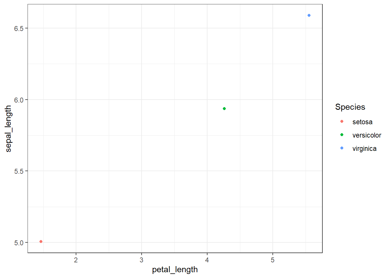

Sepal length

• Boxplot of sepal length for all species except setosa
• Boxplots need all data points (not just averages), so summarise() is not necessary (but you could filter out a specific point of the vowel)

iris %>% 
  filter(Species != "setosa") %>%
  ggplot(aes(x = Species, y = sepal_length)) +
  geom_boxplot() +
  theme_bw()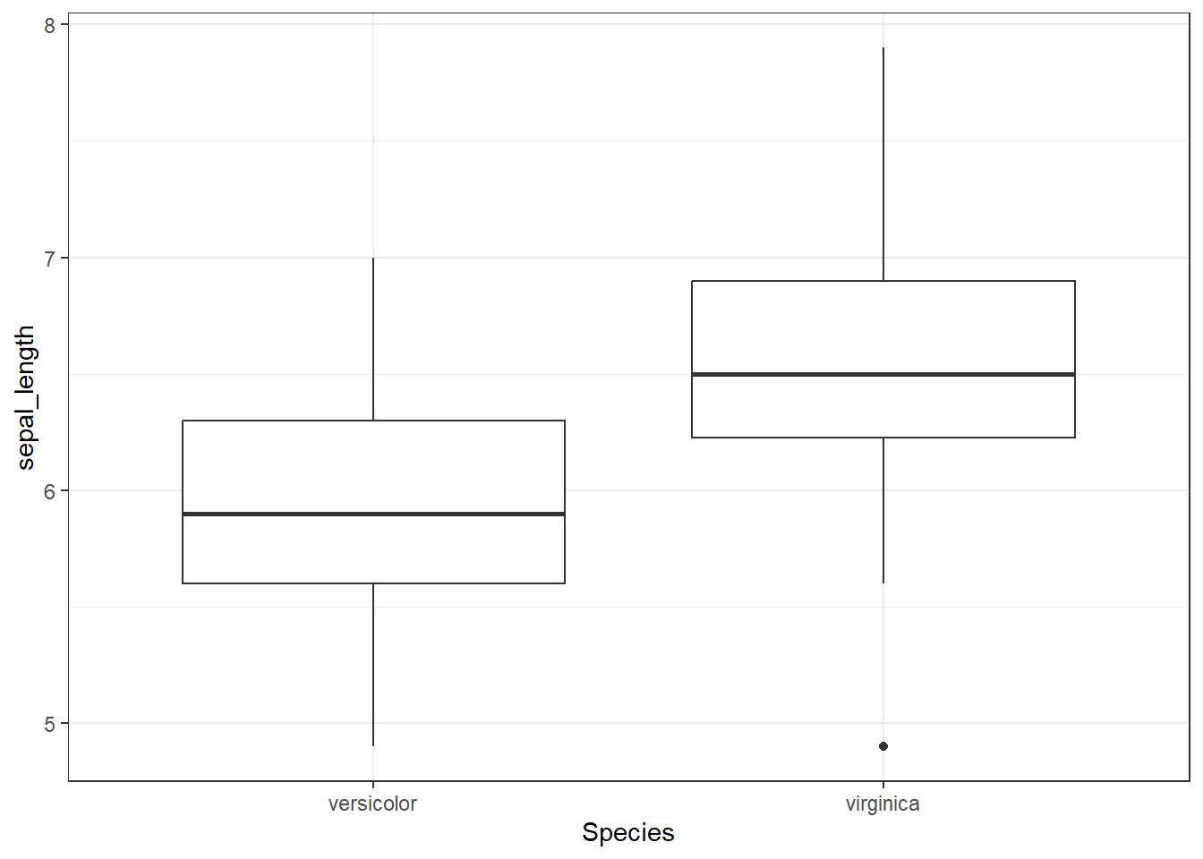

Activity 5

• Try and make your own combination of dplyr functions and ggplot