Using reposition_legend() with facets

• reposition_legend() is a function from the lemon package that lets you customise the position of a legend with more specificity than the ggplot package
• Fundamentally, it works by specifying a plot and a legend as the arguments, along with where you want the legend argument to be placed on the plot
• If you do not specify a separate legend, the function assumes that it is the legend from the specified plot
• It is especially useful for moving the legend in a plot that uses faceting. The arguments are:
  • reposition_legend(plot + facet_wrap(~ facet), 'legend_position_in_panel', panel = 'panel_where_legend_goes'
  • The argument for panel takes the form of ‘panel-column_number-row_number’
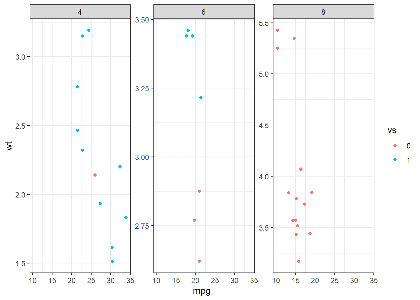
• In example below, I’ve made a scatterplot using the mtcars data set and assigned it to an object
• I have then created a facet by the cyl variable, and specified that I want the legend to be placed in the bottom right of the panel in the third column of the first row

plot <- mtcars %>% 
  mutate(across(c(vs, cyl, carb), factor)) %>% 
  ggplot()+
  geom_point(aes(x = mpg, y = wt, color = vs)) +
  theme_bw()

reposition_legend(plot + facet_wrap(~ cyl),
                  'bottom right', 
                  panel = 'panel-3-1')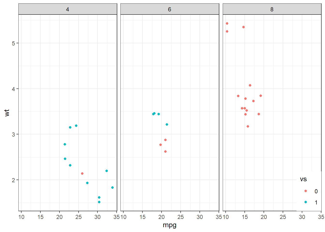

• An alternative is that I could create a two row and two column grid in the facet by specifying two rows instead of one, and then place the legend in the middle of the empty panel in the right corner

plot <- mtcars %>% 
  mutate(across(c(vs, cyl, carb), factor)) %>% 
  ggplot()+
  geom_point(aes(x = mpg, y = wt, color = vs)) +
  theme_bw()

reposition_legend(plot + facet_wrap(~ cyl, nrow = 2),
                  'center', 
                  panel = 'panel-2-2')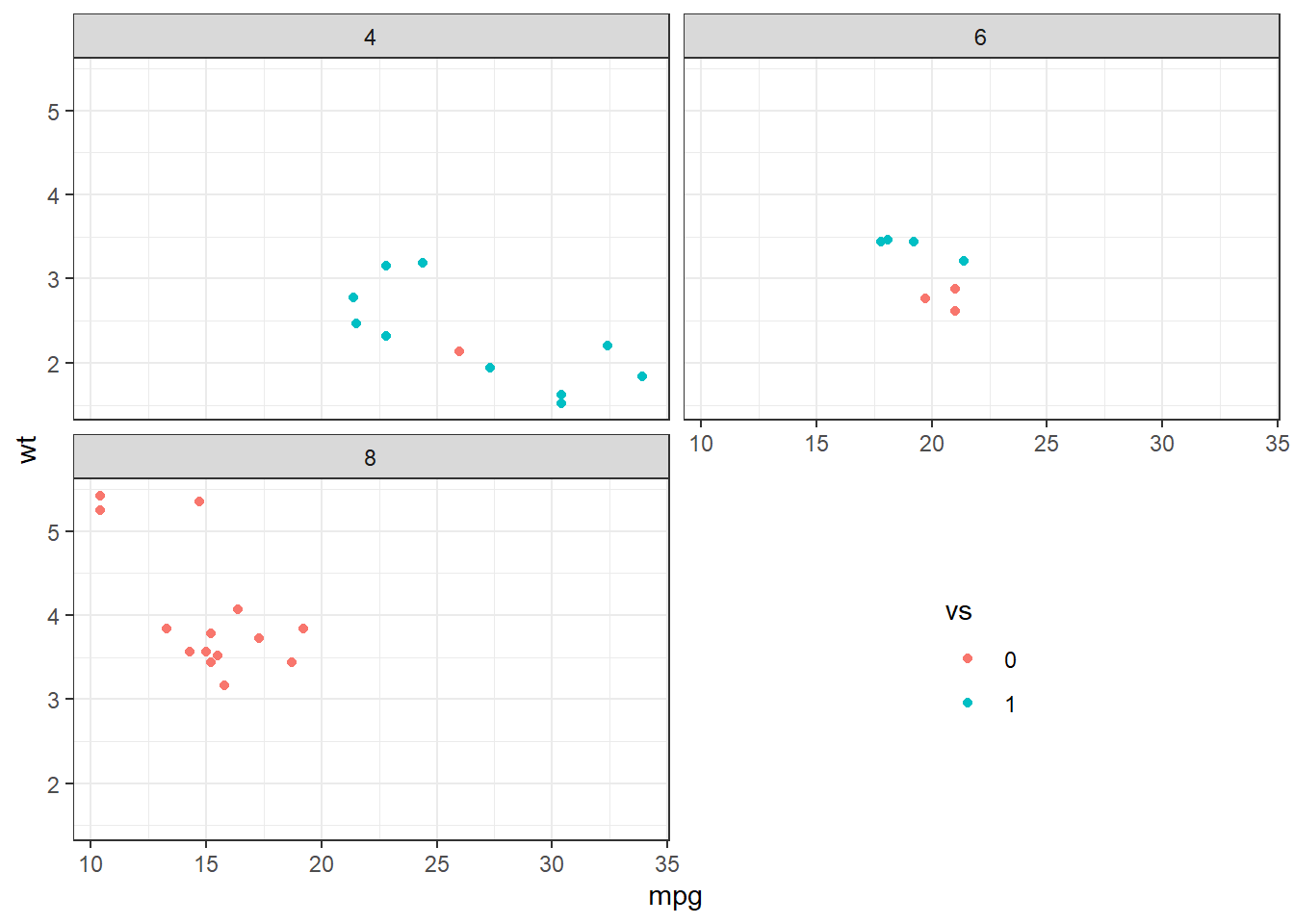

One shared legend to multiple figures

• This is an issue I’ve encountered primarily with figures generated from sjplot, because they visualise single model outputs (meaning they can’t be faceted).
• Below is an absolute hack of a solution but it’s the best I’ve got so far for visualising multiple outputs that otherwise have the same legends, but please email me if you have any suggestions!
• I have assigned each plot to an object
  • Two of the three do not have legends included
    
  • For the first one I have included the legend in the plot, and then assigned the legend only to its own object, and the plot without the legend to a separate object
    
  • Then, using plot_grid(), place the three legend-less plots next to each other, followed by the legend extracted from plot 1
    
  • The relative width argument keeps the three plots the same width, with the legend column half the width of the others
    
  • Keep in mind that each of the three plots has a different scale, which makes it look different from the facet wrap

plot1 <- mtcars %>% 
  filter(cyl == "4") %>% 
  mutate(across(c(vs, cyl, carb), factor)) %>% 
  ggplot()+
  geom_point(aes(x = mpg, y = wt, color = vs)) +
  theme_bw() #+ 
  #theme(legend.position = "none")

plot2 <- mtcars %>% 
  filter(cyl == "6") %>% 
  mutate(across(c(vs, cyl, carb), factor)) %>% 
  ggplot()+
  geom_point(aes(x = mpg, y = wt, color = vs)) +
  theme_bw() +
  theme(legend.position = "none")

plot3 <- mtcars %>% 
  filter(cyl == "8") %>% 
  mutate(across(c(vs, cyl, carb), factor)) %>% 
  ggplot()+
  geom_point(aes(x = mpg, y = wt, color = vs)) +
  theme_bw() +
  theme(legend.position = "none")

#combining plots
no_legend <- plot1 + theme(legend.position = "none")
legend <- get_legend(plot1)

#plot_grid(test_combined,legend_com,legend_ind)
plot_grid(no_legend,plot2,plot3,legend,nrow=1,rel_widths = c(1, 1,1,0.5))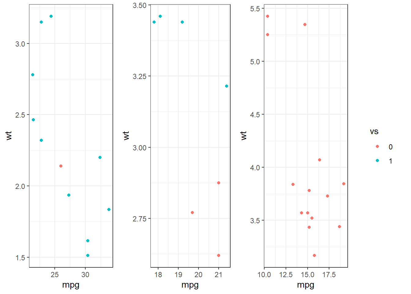

Changing the scales for facet_wrap()

The book ggplot2: Elegant graphics for data analysis explains this better than I can, but both facet_wrap() and facet_grid() have the argument ‘scales =’ which allows you to specify if you want the scales of the x and y axes to be the same (‘fixed’, the default) or change for each facet (‘free’). You can also specify only the x or y axis to be free, and the other fixed (‘free_x’ and ‘free_y’). Examples for each are provided below.

mtcars %>% 
  mutate(across(c(vs, cyl, carb), factor)) %>% 
  ggplot()+
  geom_point(aes(x = mpg, y = wt, color = vs)) +
  theme_bw()+
  facet_wrap(~ cyl) #scales = 'fixed'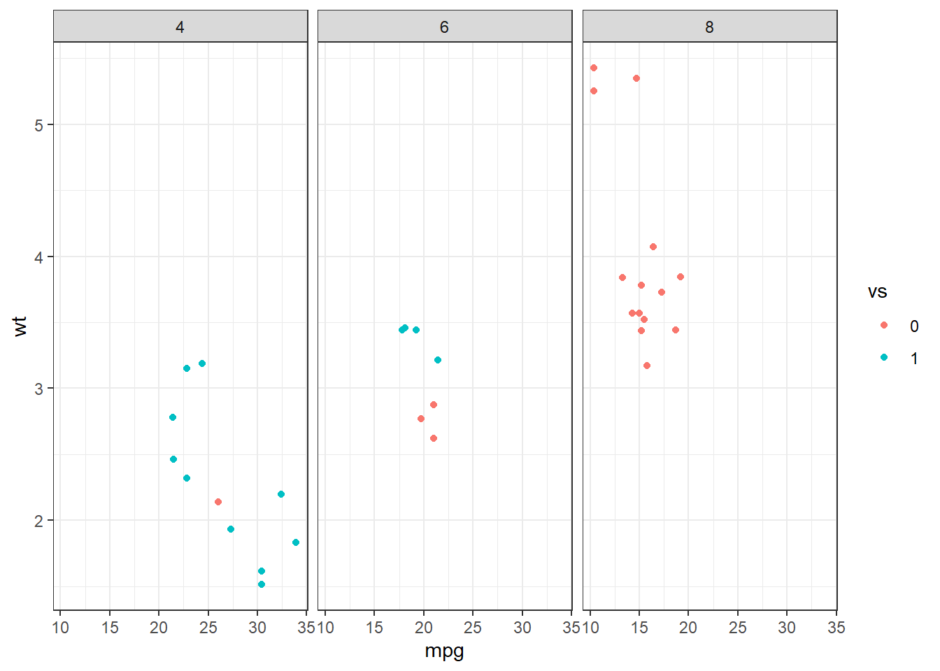

mtcars %>% 
  mutate(across(c(vs, cyl, carb), factor)) %>% 
  ggplot()+
  geom_point(aes(x = mpg, y = wt, color = vs)) +
  theme_bw()+
  facet_wrap(~ cyl, scales = 'free')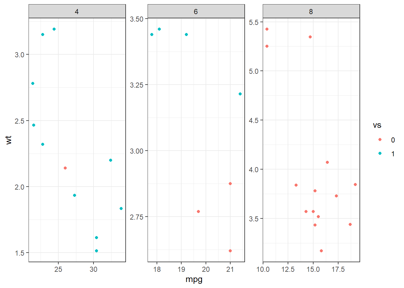 

mtcars %>% 
  mutate(across(c(vs, cyl, carb), factor)) %>% 
  ggplot()+
  geom_point(aes(x = mpg, y = wt, color = vs)) +
  theme_bw()+
  facet_wrap(~ cyl, scales = 'free_x')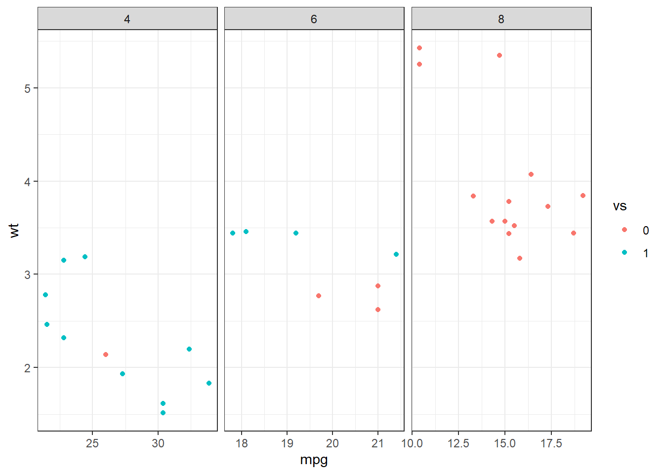 

mtcars %>% 
  mutate(across(c(vs, cyl, carb), factor)) %>% 
  ggplot()+
  geom_point(aes(x = mpg, y = wt, color = vs)) +
  theme_bw()+
  facet_wrap(~ cyl, scales = 'free_y')