Plotting an s-curve - Elena Sheard

Basic s-curve
Adding relevant labels for language change

Recently I needed to plot an s-curve and it took me an ungodly amount of time to figure out, because I don’t really understand mathematical functions.

With substantial help from stack overflow I put together this code and adjusted it for the sociolinguistics context!

library(tidyverse)

## ── Attaching packages ─────────────────────────────────────── tidyverse 1.3.2 ──
## ✔ ggplot2 3.4.1      ✔ purrr   1.0.1 
## ✔ tibble  3.1.8      ✔ dplyr   1.0.10
## ✔ tidyr   1.3.0      ✔ stringr 1.5.0 
## ✔ readr   2.1.3      ✔ forcats 1.0.0 
## ── Conflicts ────────────────────────────────────────── tidyverse_conflicts() ──
## ✖ dplyr::filter() masks stats::filter()
## ✖ dplyr::lag()    masks stats::lag()

library(scales)

## 
## Attaching package: 'scales'
## 
## The following object is masked from 'package:purrr':
## 
##     discard
## 
## The following object is masked from 'package:readr':
## 
##     col_factor

Basic s-curve

The basic s-curve maps a particular function with stat_function() added to a ggplot object. I can’t explain much more about the function aside from the larger the numbers in x the steeper the line and the more plateau you get at either end of the curve.

#s-curve
p <- ggplot(data = data.frame(x = c(-8, 8)), aes(x))

p +
  stat_function(fun = function(x) exp(x)/(1 + exp(x)), n = 100) +
  theme_bw(base_size = 14)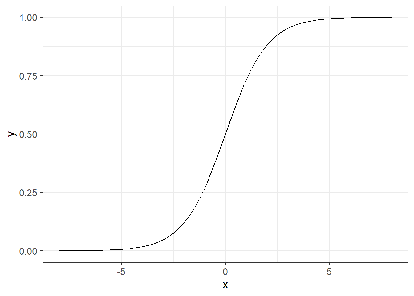

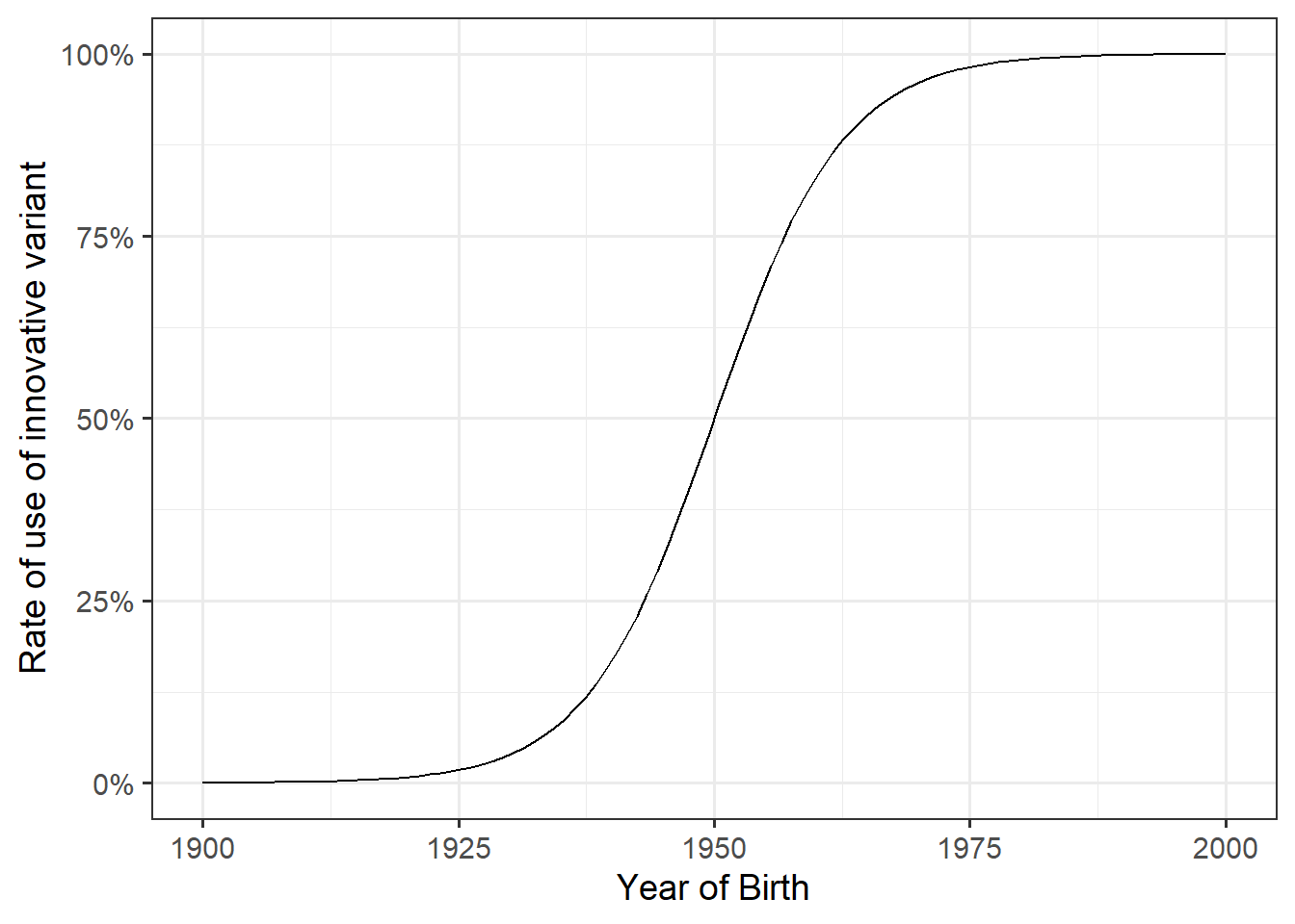
Adding relevant labels for language change

To relate the curve to language change I used labs() to change the x and y axis labels to “Year of Birth” (corresponding to older speakers born longer ago and younger speakers born more recently) and “Rate of use of innovative variant”. I also changed the labels of the breaks on the x axis to every 25 years starting from 1900 with scale_x_continuous(). Finally, I just changed the y axis to % using scale_y_continuous() and the scales package.

p <- ggplot(data = data.frame(x = c(-8, 8)), aes(x))

p +
  stat_function(fun = function(x) exp(x)/(1 + exp(x)), n = 100) +
  labs(x = "Year of Birth",
       y = "Rate of use of innovative variant") +
  scale_x_continuous(breaks = c(-8, -4, 0, 4, 8),
                     labels = c('1900', '1925', '1950',
                                '1975', '2000')) + 
  scale_y_continuous(labels = percent) +
  theme_bw(base_size = 14)